3.1 Support Vector Machines

Support Vector Machines (SVMs) were introduced by Vapnik [54] based on the structural risk minimization (SRM) principle, as an alternative to the traditional empirical risk minimization (ERM) principle. The main idea is to find a hypothesis h from a hypothesis space H for which one can guarantee the lowest probability of error Err(h). Given a training set of n examples:

(3.2)

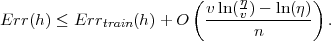
SRM connects the true error of a hypothesis h with the error on the training set, Err_train, and with the complexity of the hypothesis (3.3):

(3.3)

This upper bound holds with a probability of at least 1 - η. v denotes the VC-dimension¹ [54], which is a property of the hypothesis space H and indicates its expressiveness. This bound reflects the tradeoff between the complexity of the hypothesis space and the training error , i.e a simple hypothesis space will not approximate the desired functions, resulting in high training and true errors. On the other hand, a too-rich hypothesis space, i.e. with large VC-dimension, will result in overfitting. This problem arises because, although a small training error will occur, the second term in the right-hand side of (3.3) will be large. Hence, it is crucial to determine the hypothesis space with the sufficient complexity. In SRM this is achieved by defining a nested structure of hypothesis spaces H_i, so that their respective VC-dimension v_i increases:

(3.4)

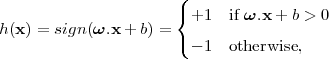
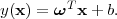
This structure is apriori defined to find the index for which (3.3) is minimum. To build this structure the number of features is restricted. SVMs learn linear threshold functions of the type:

(3.5)

where ω = (ω₁,ω₂,…,ω_N)^T are linear parameters (weights) of the model and b is the bias. Linear threshold functions with N features have a VC-dimension of N+1 [54].

3.1.1 Linear hard-margin SVMs

In the simplest SVM formulation, a training set can be separated by at least one hyperplane, i.e. data are linearly separable and a linear model can be used:

(3.6)

In this case, SVMs are called linear hard-margin and there is a weight vector ω′ and a threshold b′ that correctly define the model. Basically there is a function of the form (3.6) that satisfies y(x_i) > 0 for samples with t_i = 1 and y(x_i) < 0 for points having t_i = -1, so that for each training data point (x_i,t_i)

(3.7)

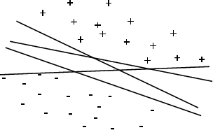
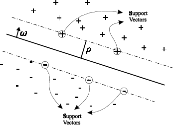
As a rule there can be multiple hyperplanes that allow such separation without error (see Figure 3.1), and the SVM determines the one with largest margin ρ, i.e. furthest from the hyperplane to the closest training examples. The examples closer to the hyperplane are called support vectors (SVs) and have an exact distance of ρ to the hyperplane. Figure 3.2 depicts an optimal separating hyperplane and four SVs.

The perpendicular distance of a point from a hyperplane defined by y(x) = 0, where y(x) takes the form of (3.6), is given by [7]. As we are only interested in solutions for which all samples are correctly classified, so that t_iy(x_i) > 0, the distance of a single data point x_i to the decision surface is given by

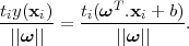(3.8)

The margin is then given by the perpendicular distance to the closest point x_i of the data set, and we wish to optimize the parameters ω and b in order to maximize this distance. Thus, the maximum margin solution is found by solving

(3.9)

Using a canonical representation of the decision hyperplane, all data points satisfy

(3.10)

When the above equality holds, the constraints are said to be active for that data point, while for the rest the constraints are inactive. There will be always at least one active constraint, since there will always be a closest point, and once the margin has been maximized, there will be at least two active constraints. Then, the optimization problem consists of maximizing ||ω||^-1, which is equivalent to minimizing ||ω||², and so we have to solve the (primal) optimization problem:

(3.11)

These constraints establish that all training examples should lie on the correct side of the hyperplane. Using the value of 1 on the right-hand side of the inequalities enforces a certain distance from the hyperplane:

(3.12)

where ||ω|| denotes the L₂-norm of ω. Therefore minimizing ω.ω is equivalent to maximizing the margin. The weight vector ω and the threshold b describe the optimal (maximum margin) hyperplane.

Vapnik [54] showed there is a relation between the margin and the VC-dimension. Considering the hyperplanes h(x) = sign(ω.x + b) in an N-dimensional space as a hypothesis, if all examples x_i are contained in a hyper-circle of diameter R, it is required that, for examples x_i:

(3.13)

and then this set of hyperplanes has a VC-dimension, v, bounded by:

(3.14)

where [c] denotes the integer part of c. Thus, the VC-dimension is smaller as the margin becomes larger. Moreover, the VC-dimension of the maximum margin hyperplane does not necessarily depend on the number of features, but on the Euclidean length ||ω|| of the weight vector optimized by the SVM. Intuitively this means that the true error of a separating maximum margin hyperplane is close to the training error even in high-dimensional spaces, as long as it has a small weight vector.

The primal constrained optimization problem (3.11) is numerically difficult to handle. Therefore, one introduces Lagrange multipliers, α_i ≥ 0, with one multiplier for each of the constraints in (3.11), obtaining the Lagrangian function

(3.15)

where α = (α₁,…,α_n)^T . Note the minus sign in front of the Lagrangian multiplier term, because we are minimizing with respect to ω and b, and maximizing with respect to α. Setting the derivatives of L(ω,b,α) with respect to ω and b to zero, we obtain the following two conditions:

(3.16)

(3.17)

Eliminating ω and b from L(ω,b,α) gives the dual representation of the maximum margin problem

(3.18)

The matrix Q with Q_ij = t_it_j(x_i.x_j) is commonly referred to as the Hessian matrix. The result of the optimization process is a vector of Lagrangian coefficients α = (α₁,…,α_n)^T for which the dual problem (3.18) is optimized. These coefficients can then be used to construct the hyperplane, solving the primal optimization problem (3.11) just by linearly combining training examples (3.19).

(3.19)

Only support vectors (SVs) have a non-zero α_i coefficient. To determine b from (3.18) and (3.19), an arbitrary support x_SV vector with its class label t_SV can be used.

3.1.2 Soft-margin SVMs

Hard-margin SVMs fail when the training data are not linearly separable, since there is no solution to the optimization problems (3.11) and (3.18). Most pattern classification problems are not linearly separable, thus it is convenient to allow misclassified patterns, as indicated by the structural risk minimization [54]. The rationale behind soft-margin SVMs is to minimize the weight vector, like the hard-margin SVMs, but simultaneously minimize the number of training errors by the introduction of slack variables, ξ_i. The primal optimization problem of (3.11) is now reformulated as

(3.20)

If a training example is wrongly classified by the SVM model, the corresponding ξ_i will be greater than 1. Therefore ∑ _i=1ⁿξ_i constitutes an upper bound on the number of training errors. The factor C in (3.20) is a parameter that allows the tradeoff between training error and model complexity. A small value of C will increase the training errors, while a large C will lead to behavior similar to that of a hard-margin SVM.

Again, this primal problem is transformed in its dual counterpart, for computational reasons. The dual problem is similar to the hard-limit SVM (3.18), except for the C upper bound on the Lagrange multipliers α_i:

(3.21)

As before, all training examples with α_i > 0 are called support vectors. To differentiate between those with 0 ≤ α_i < C and those with α_i = C, the former are called unbounded SVs and the latter are called bounded SVs.

From the solution of (3.21) the classification rule can be computed exactly, as in the hard-margin SVM:

(3.22)

The only additional restriction is that the SV (x_SV ,t_SV ) for calculating b has to be an unbounded SV.

3.1.3 Nonlinear SVMs

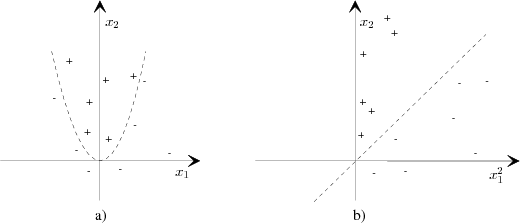
Linear classifiers are inappropriate for many real-world problems, since the problems have inherently nonlinear structure. A remarkable property of SVMs is that they can easily be transformed into nonlinear learners [9]. The attribute data points x are mapped into a high-dimensional feature space X′. Despite the fact that the classification rule is linear in X′, it is nonlinear when projected into the original input space. This is illustrated with the following example consisting of a vector x = (x₁,x₂), with two attributes x₁ and x₂. Let us choose the nonlinear mapping:

(3.23)

Although it is not possible to linearly separate the examples in Figure 3.3a), they become linearly separable in Figure 3.3b), after the mapping with Φ(x) into the higher dimensional feature space.

In general, such a mapping Φ(x) is inefficient to compute. There is a special property of SVMs that handles this issue. During both training and testing, it is sufficient to be able to compute dot-products in feature space, i.e. Φ(x_i).Φ(x_j). For special mappings Φ(x) such dot-products can be computed very efficiently using kernel functions K(x₁,x₂). If a function K(x₁,x₂) satisfies Mercer’s Theorem, i.e. it is a continuous symmetric kernel of a positive integer operator, it is guaranteed to compute the inner product of the vectors x₁ and x₂ after they have been mapped into a new space by some nonlinear mapping Φ [54]:

(3.24)

Depending on the choice of kernel function, SVMs can learn polynomial classifiers (3.25), radial basis function (RBF) classifiers (3.26) or two-layer sigmoid neural networks (3.27).

(3.25)

(3.26)

(3.27)

The kernel K_poly(x₁,x₂) = (x₁.x₂ + 1)² corresponds to the mapping in Equation (3.23). To use a kernel function, one simply substitutes every occurrence of the inner product in equations (3.21) and (3.22) with the desired kernel function.