Tool Views (Images):
Main
page (Menu)
![]()
Fig.1: General view. There are three linked views: Microarray on the
lower left side, scatter plot and parallel coordinates
on the lower right side. Go to
top…
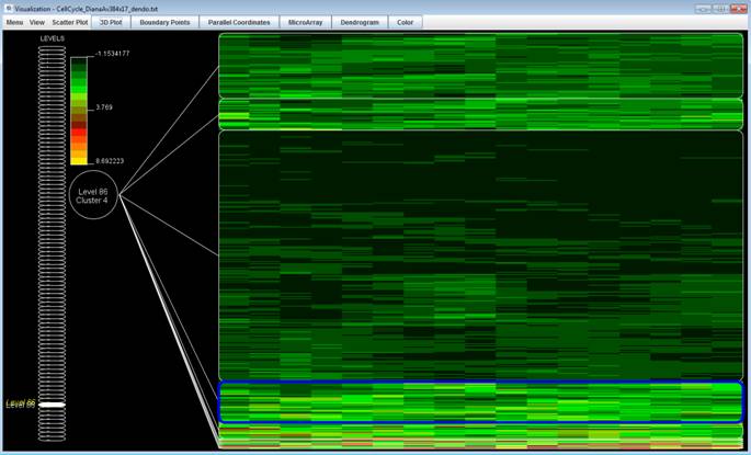
Fig. 2: Main window of the
tool, on the left side, the levels of the dendrogram can be chosen and on the
right side, all clusters of the current
level are shown. Go to
top…
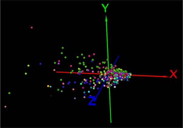
Fig. 3: 3D scatter plot with
correlation analysis. Each cluster of the level chosen in the main view is
represented
with a different color. Go to top…
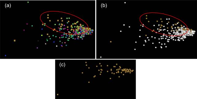
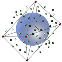
Fig. 4: a) Compares
the current cluster by changing the shape of the points (cubes) vs. the
remaining points of the data set;
b) compares the
current cluster (colored) vs. the remaining points of
the data set (white circle) and c) displays only the current cluster.
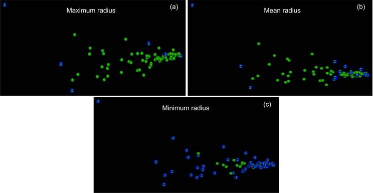
Fig. 5: Shows the options for
boundary points; a) displays the boundary points computed with maximum radius;
b) displays the boundary
points computed with mean
radius; and c) displays the boundary points computed with minimum radius. Go to
top…
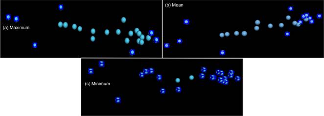
Fig. 6: Displays the boundary
points of a cluster computed with maximum, mean and minimum radius. Go to
top…
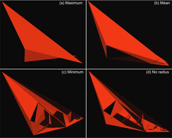
Fig. 7: Shows the solid
surface of the cluster chosen in Fig. 5. a) radius
maximum, b) radius mean, c) radius minimum and d) no radius.
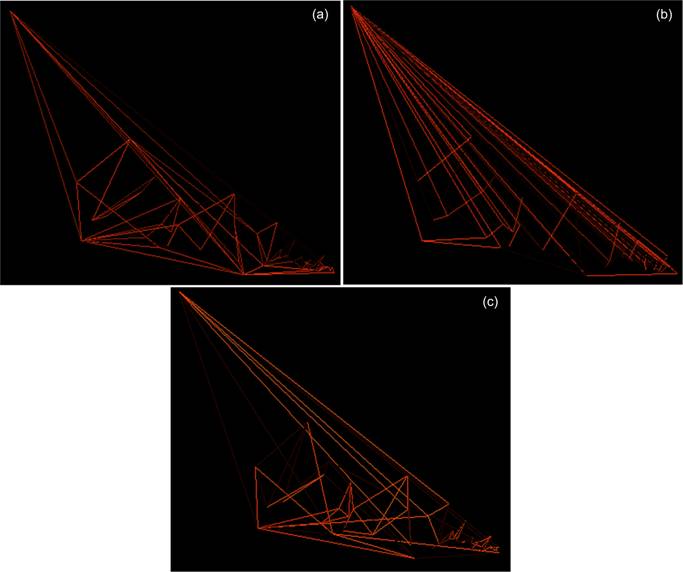
Fig. 8: Shows the shape of the
cluster (Fig. 7) through lines, built with minimum radius for three types of
triangulations a), b) and c).
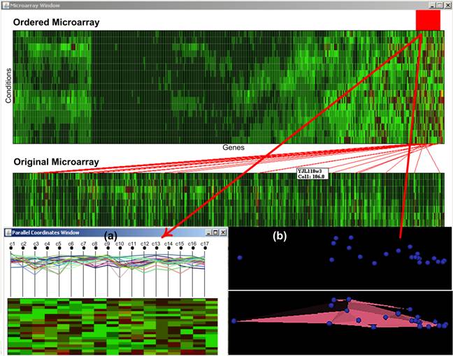
Fig. 9: Shows the original and
ordered microarray, the chosen cluster (in red) on the ordered microarray is
zoomed and displayed as
parallel coordinates in a).
b) shows the points and the surface of the chosen
cluster on the scatter plot. Go to top…
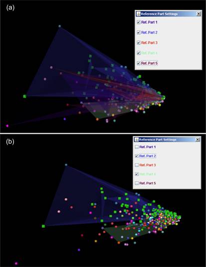
Fig. 10: Displays the loaded
Reference Partition; a) shows the data set with the reference partition, each
partition with a different color;
b) shows
the same but filtering some surfaces of the reference partition. Go to
top…
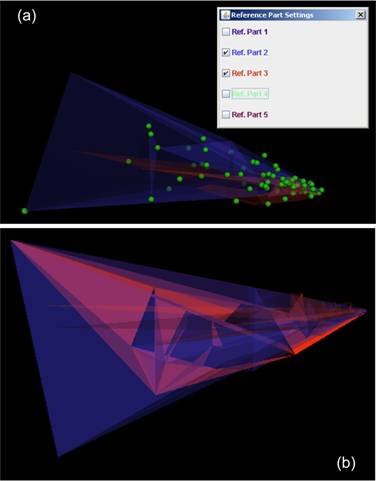
Fig. 11: a) Displays two
partitions that agree with the cluster; b) compares the two partitions with the
cluster in form of surface.
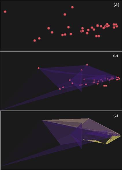
Fig. 12: a) Displays
the points of a cluster; b) displays the partition-surface that better agrees
with the cluster; c) compares the partition-surface
with the cluster
surface. Go to top…
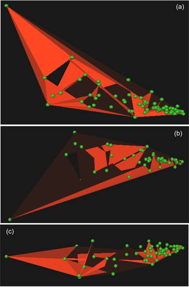
Fig. 13: Shows different views
of the solid built from a cluster (Fig. 7), including all points bellowing to
the cluster.
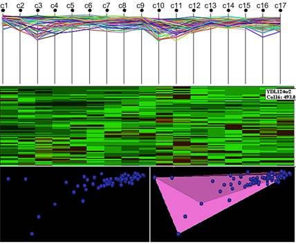
Fig. 14: Shows a cluster by
four different ways: as microarray,
parallel coordinates, points and
surface on the scatter
plot. Go to top…